
Overview
Discrete choice models have been used extensively in economics, marketing, and transportation research. In this competition, we aim to predict the choice among bundles of safety features in cars. The choice-based conjoint data was collected by General Motors to understand consumers' trade-offs for various vehicle features.
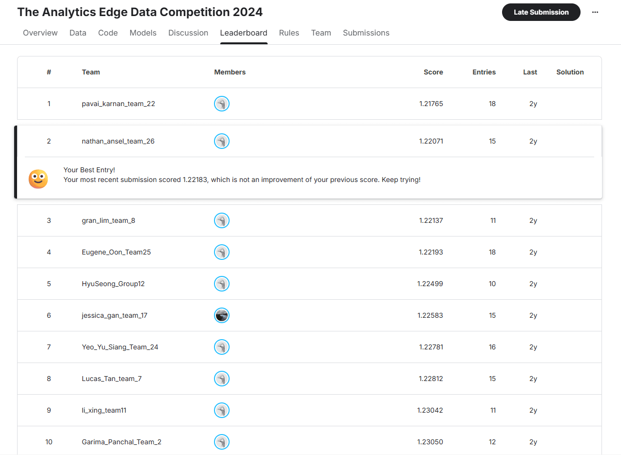
Our team of 4 developed both classical discrete-choice models and modern ML methods in R: Multinomial Logit (MNL), Random Forest, and XGBoost, validated with 5-fold cross-validation and combined via a weighted soft-voting ensemble. Across 15 submissions, our best soft-voting ensembles placed us 1st runner-up (2nd overall) on the competition's leaderboard.
GitHub - nathanansel28/tae-hackathon
Full R codebase: EDA, all base models, submission pipeline, ensemble weight tuning, and a reproducible renv environment.
github.com
Methodology
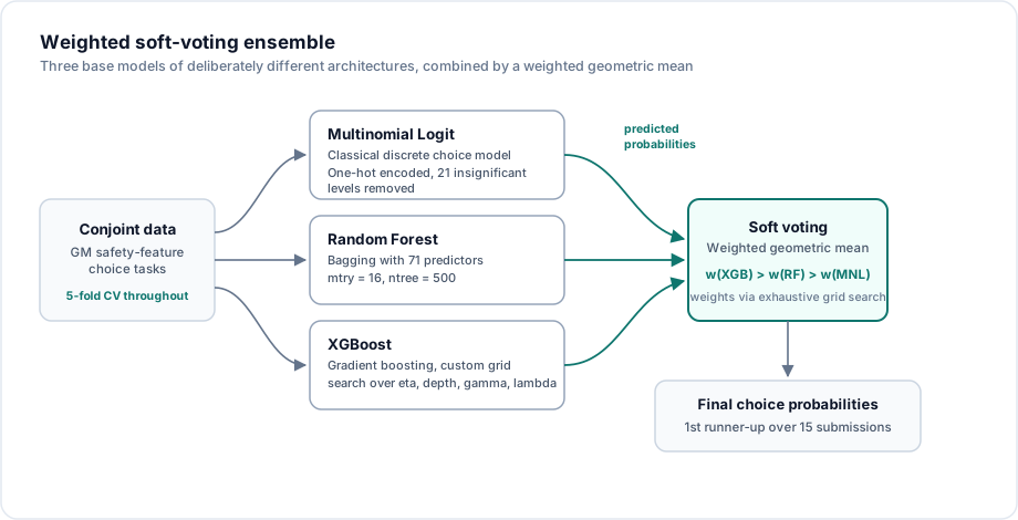
We split our effort into two tracks: classical models grounded in discrete choice theory, and modern ML methods with strong Kaggle track records. Each track produced one or more base models, whose predicted probabilities were then combined by a weighted soft-voting ensemble:
Discrete Choice Theory
The main reference for interpreting the data was Mishra, Natarajan et al.'s paper on marginal distribution choice models, which also highlighted feature engineering via one-hot encoding and feature selection via parameter significance. We tested three classical models: Nested Logit (relaxes the Independence of Irrelevant Alternatives assumption) and Mixed Logit (models random taste variation) to capture consumer heterogeneity, plus the simpler MNL, which assumes homogeneity. All three performed similarly, so we selected MNL for its simplicity and comparable log-loss.
We one-hot encoded the safety features (since feature levels aren't inherently ordered) and avoided the dummy variable trap by dropping one level per categorical variable. This paid off concretely: several encoded levels (e.g. AF3, BU6) turned out statistically insignificant while other levels of the same feature were significant, a distinction a non-encoded model would have missed. The final MNL model removed 21 such insignificant variables.
Boosting: XGBoost
We chose XGBoost over alternatives like AdaBoost, CatBoost, and LightGBM for its computational efficiency and ease of tuning. Feature engineering removed three groups of variables before training: task/case/number indices (uninformative row identifiers), redundant demographic categoricals (already represented as encoded indices elsewhere), and all "choice 4" (no selection) indicator features, which are always zero by construction.
Hyperparameters were tuned via a self-implemented grid search (rather than a built-in one, so we could track our own log-loss/accuracy/overfitting metrics directly), fine-tuning number of trees, learning rate (eta), max tree depth, minimum loss reduction (gamma), and L2 regularization (lambda), each evaluated for its own overfitting/underfitting trade-off. 5-fold cross-validation was used throughout to keep tuning decisions consistent across folds.
Bagging: Random Forest
Our Random Forest model used the same encoded safety features plus 11 alternative-specific effects (e.g. income, age, region, park access), for 71 predictor variables in total. We tuned mtry (variables considered per split) to 16 via tuneRF(), double the default of 8, and swept ntree from 500 to 700, settling on 500 as the best balance between capturing enough signal and avoiding overfitting on a large dataset.
Ensembling: Soft Voting Classifier
Rather than layering a meta-learner on top of the three base models (a classic stacking approach), we deliberately chose a simpler soft voting classifier: a weighted geometric mean of the XGBoost, MNL, and RF predicted probabilities. We preferred this over an additional meta-learner because model complexity increases while interpretability decreases, with no guarantee the meta-learner generalizes to unseen data.
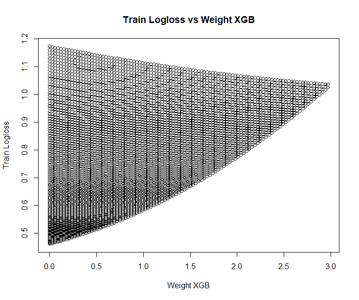
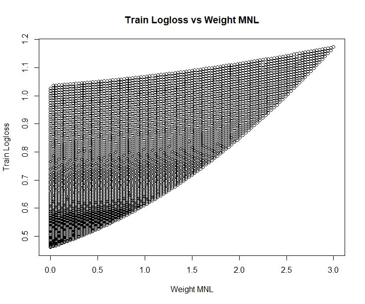
Ensemble weights were tuned via an exhaustive grid search. The sweep told a consistent story: increasing the XGBoost or RF weight decreased log-loss, while increasing the MNL weight increased it, so the final ensemble weighted XGBoost highest, followed by RF, then MNL.
Results
We made 15 submission attempts overall, tracking train/test log-loss locally alongside the competition's public and private leaderboard scores.
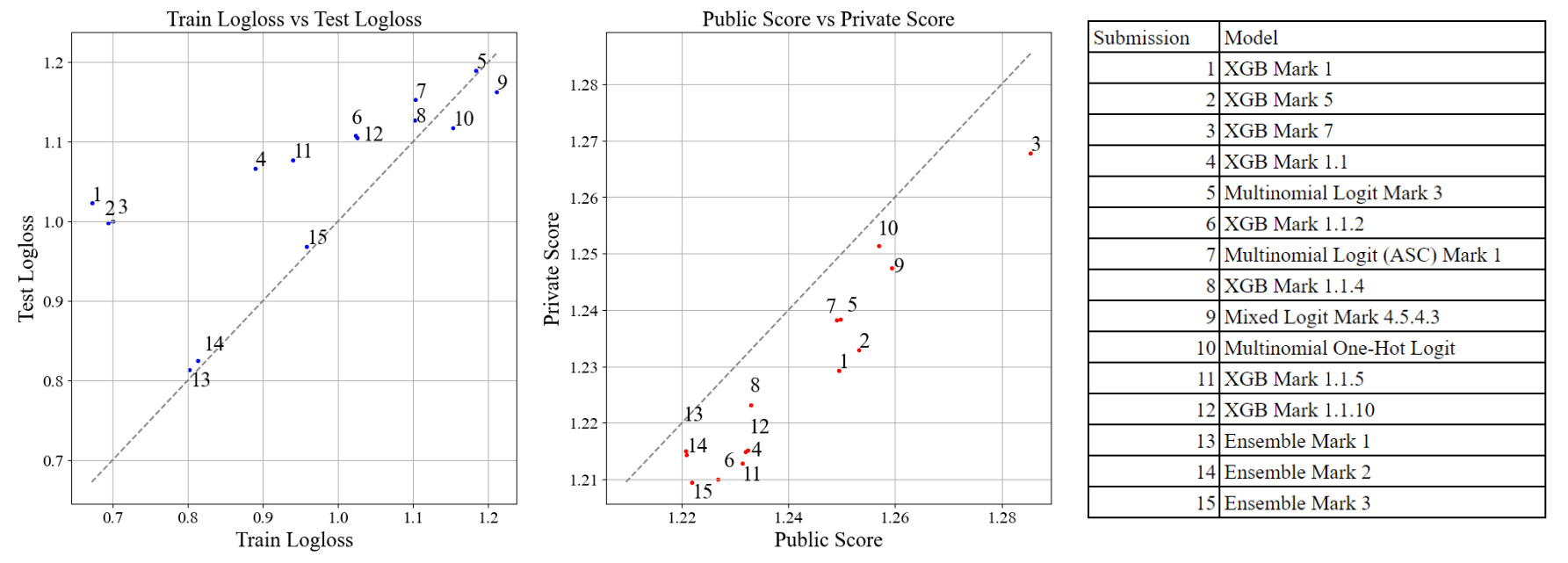
A key lesson: extremely low log-loss on its own wasn't a reliable signal. One high-variance model (model 3) scored well on training data but poorly on both leaderboards (overfitting), while another (model 5) with a small train/test gap still underperformed because its log-loss was high from the start. The strongest submissions, the soft-voting ensembles (models 13-15), balanced both minimizing log-loss and keeping the train/test gap small.
Interpretability
Beyond raw predictive performance, we spent real effort interpreting what each model learned:
- MNL coefficients are directly interpretable: positive coefficients mean a feature is desirable to customers, negative means undesirable. Unsurprisingly, price carries a negative coefficient while most safety features carry positive ones.
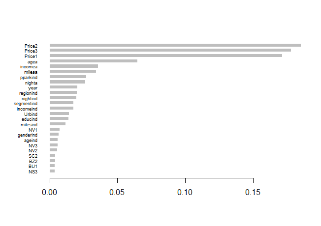
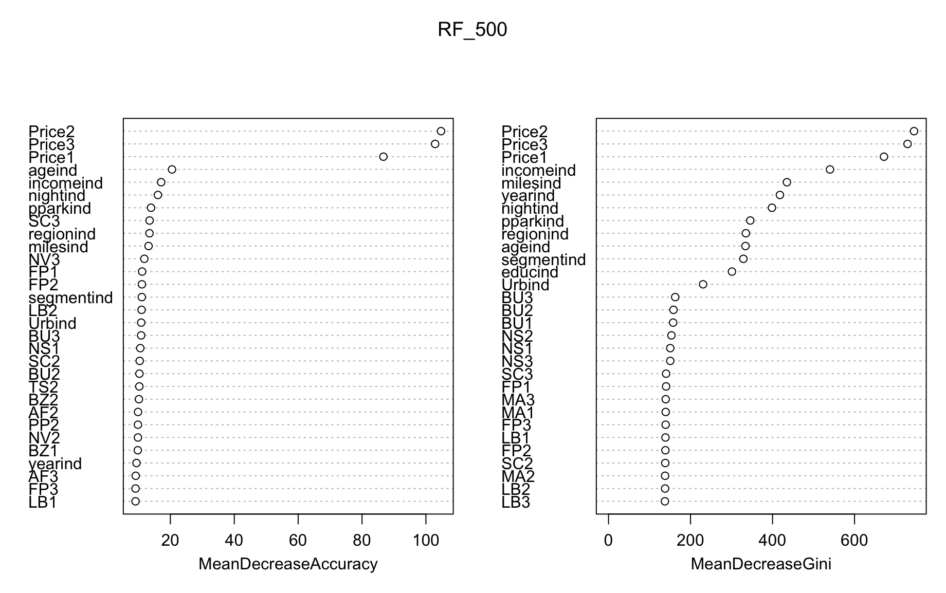
- Random Forest variable importance (via
varImp()) showed the three Price levels far outweighing every other feature, followed by alternative-specific effects like income and age.
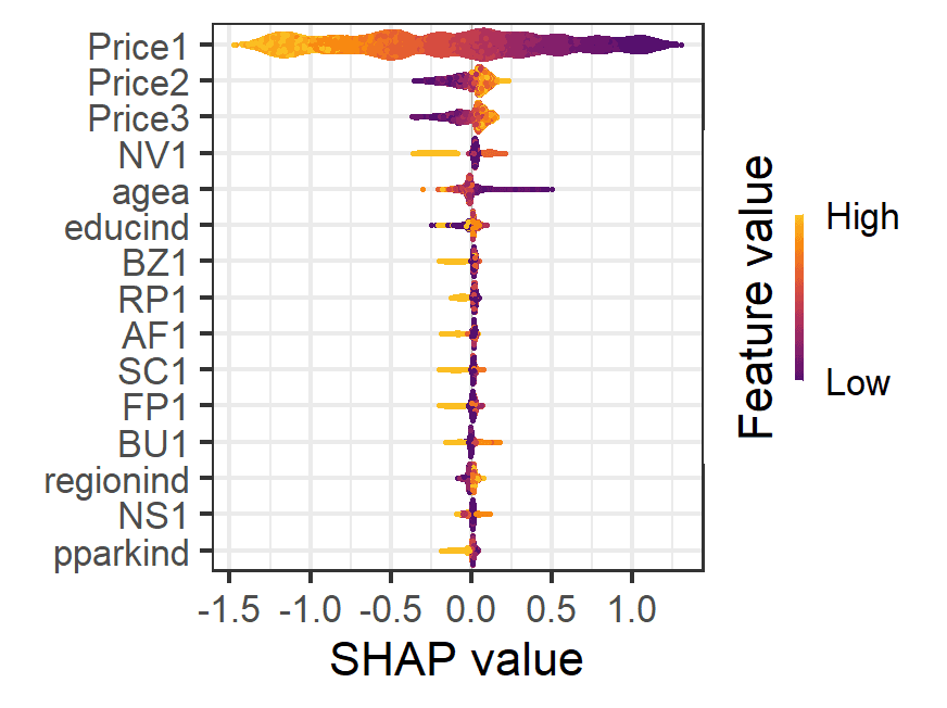
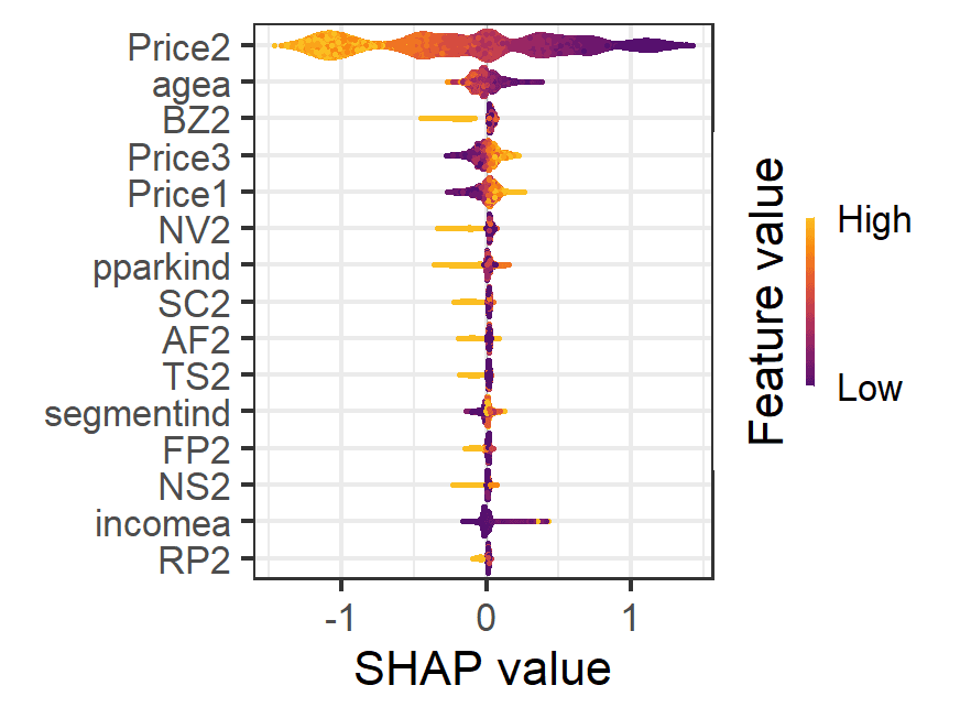
- SHAP values on the XGBoost model confirmed the same story from a different angle: regardless of which package a customer chose, its Price feature was consistently the most influential factor in that decision.
Limitations & Further Research
Our self-implemented grid search was time-consuming given the large hyperparameter space, and remained prone to overfitting the training set even with cross-validation. Bayesian optimization (e.g. via ParBayesianOptimization or MlBayesOpt in R) would likely have searched the space more efficiently. We also deliberately scoped out deep learning approaches in favor of theory-grounded choice models and Kaggle-proven ML methods. With access to larger discrete-choice datasets, though, DL methods capable of learning hidden distributions beyond what classical choice models can capture are a promising direction for future work.