
Overview
Assembly line scheduling looks like a simple question: given a Bill-of-Materials, when should each operation run, on which machine? Underneath, it sits on top of a combinatorial explosion. The number of feasible schedules grows exponentially in the number of operations and workcentres, and the problem is NP-hard. Exact methods can, in principle, return the optimum; in practice they time out long before reaching the problem sizes a real factory cares about.
This was a 14-week project for 40.014 Engineering Systems Architecture and 40.012 Manufacturing & Service Operations, delivered by a 7-person team against the mission statement:
"Develop an intuitive and efficient web application using heuristic methods to optimise large-scale assembly line scheduling for manufacturing companies, tailored to their specific objectives."
The multi-objective nature of the problem means that production managers don't all want the same thing: makespan, work-in-progress (WIP) cost, number of tardy jobs, and algorithm runtime all trade off against one another. Rather than pick a winner on their behalf, we shipped four heuristics and let the user choose the objective.
Heuristics engine on GitHub
LETSA, EDD, Simulated Annealing, and Lagrangian Relaxation, plus the data generator and 1,944-case benchmark harness.
github.com
GANTT. web app on GitHub
React frontend and FastAPI backend.
github.com
My role
I implemented all four heuristics and owned the Python backend and the benchmarking harness; I contributed to the React frontend, which was primarily the work of other teammates.
Why heuristics, and which four
The design space was wide: we reviewed nine candidate methods in Report 1, including Shifting Bottleneck, memetic and genetic algorithms, Variable Neighbourhood Search, Multi-type Particle Swarm Optimisation, and Tabu Search. We narrowed to four, chosen so that each one earns its place against a different objective rather than four variations on the same idea:
- LETSA (Lead Time Evaluation and Scheduling Algorithm, from Agrawal et al.) builds a schedule backwards from the final assembly, repeatedly scheduling operations on a dynamically recomputed critical path. Targets makespan and WIP cost simultaneously: scheduling just-in-time means components aren't sitting in inventory waiting for their parent operation.
- EDD (Earliest Due Date / Moore–Hodgson) is the classical rule for minimising the number of tardy jobs. The textbook version is single-machine; our implementation extends it to a multi-machine setting under BOM precedence constraints, which is the part that actually took work.
- Simulated Annealing is a metaheuristic for makespan, accepting non-improving moves with a temperature-controlled probability so the search can climb out of local optima that a greedy rule would be trapped in.
- Lagrangian Relaxation follows Xu & Nagi's approach: formulate the problem as a MILP, dualise the hard constraints into the objective with Lagrange multipliers, and solve the decomposed subproblems. Fast, but its real value is different, and it's the reason the rest of this page has numbers in it.
The bit that makes the benchmark honest
A heuristic returns a schedule. On its own, that number is meaningless: a makespan of 340 is only good or bad relative to what was achievable. Most coursework projects stop here and compare heuristics against each other, which tells you the ranking but never the distance from optimal.
Lagrangian Relaxation solves that. Because relaxing constraints can only improve the objective, the relaxed solution is a valid lower bound on the true optimum , while any feasible schedule from a heuristic is an upper bound:
which gives every other heuristic a certificate of quality:
So LR pays for itself twice: it's a competitive heuristic in its own right, and it's the yardstick the other three are measured against. Without it we'd be reporting a leaderboard; with it we're reporting how close to optimal each schedule actually is.
Benchmarking at scale: 1,944 test cases
Anecdotal results on a handful of BOMs are how you convince yourself of something false. I built a parameterised data generator (following the methodology of Hall & Posner, 2001) and swept it systematically:
| Parameter | Meaning | Values |
|---|---|---|
| Operations in the BOM (problem size) | 15, 30 (small) · 50, 100 (medium) · 200 (large) · 500 (stress) | |
| BOM network density: high gives a long, deep BOM; low gives a wide, shallow one | 0.1, 0.5, 0.9 | |
| Logarithmic distribution parameter for processing times: higher means higher variance | 0.15, 0.95 | |
| Distinct machines required across all operations | ||
bottleneck | Whether a machine is designated a bottleneck | true / false |
On top of the BOM parameters, factory capacity was varied across three scenarios reflecting real industrial conditions: abundant machines per workcentre (heavy parallelism), mild capacity (uneven across workcentres), and one machine per functionally identical machine type in the BOM, which is the adversarial case where scheduling is hardest and the optimal makespan is most difficult to approach.
The cross-product yielded 1,944 test cases. Heuristics were also validated against two external datasets (a multi-objective flexible job shop cell benchmark, and a remanufacturing system scheduling dataset), so we weren't only testing against our own generator's biases.
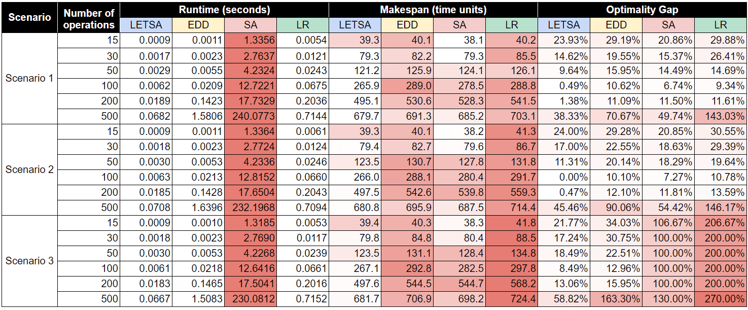
Results, including the ones we didn't expect
LETSA won outright: best makespan and fastest runtime. That's an uncomfortable result for a team that had just spent weeks implementing a metaheuristic: Simulated Annealing came second on solution quality while costing substantially more compute. SA's ability to escape local optima simply didn't buy enough on this problem structure to beat a well-designed critical-path heuristic. EDD and LR were near-instantaneous but carried visibly wider optimality gaps, which is exactly what you'd expect from a dispatching rule and a dualised bound.
On performance requirements: we had committed in Report 1 to a 30-minute ceiling for BOMs of up to 200 operations. Every heuristic terminated within 30 seconds at that size, roughly two orders of magnitude inside the requirement. The 500-operation cases were run purely as a stress test, beyond the stated requirement envelope.
We kept all four heuristics in the shipped product anyway. A production manager staring at a single number has no way to sanity-check it; a production manager looking at four schedules, their objective trade-offs, and an optimality gap against a mathematically valid lower bound can make an informed decision. That's the difference between a solver and a decision-support tool.
From solver to product
Sitting in a Jupyter notebook, the heuristics are useless to their actual users: production managers, not data scientists. So we shipped GANTT., a web app that separates concerns cleanly across two services:
- Backend: Python, FastAPI served under Uvicorn, exposing the heuristic engine over a REST interface. CSV BOM upload, objective selection, schedule generation, and the resulting schedule returned as structured data.
- Frontend: React, with Ant Design and MUI components and
timelines-chartsfor Gantt rendering. Everything (instructions, upload, objective choice, Gantt output) lives on a single manage page with a sticky stepper, so users never lose their place mid-flow. The layout collapses from horizontal to vertical below 800px.
Limitations
- Heuristics, not optima. Every schedule we produce is near-optimal by construction. The LR bound tells us how near, but a parallel team running exact methods would beat us on small instances, and should.
- The generator is ours. 1,944 cases sweep a wide parameter space, but they're synthetic. The two external benchmark datasets partially cover this, though neither is a live factory BOM.
- SA was under-tuned. Its cooling schedule is the single largest lever on its performance, and we did not tune it exhaustively. LETSA beat it, but I'd want to re-run that comparison with a properly annealed schedule before treating the result as settled.